 |
The Graphical Query Language: |
Tutorial GQLCluster
Overview
GQLCluster is a tool for performing cluster and mixture estimation analysis from time course data. It provides a range of methods to: pre-process the data, obtain a initial collection of HMMs, estimate mixtures of time courses and to infer groups of them, to visualize the results and to elucidate them in context to other biological information.
Getting Started
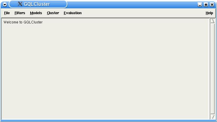
Run GQLCluster with the following command (or by double-clicking at the executable binary file):
python GQLCluster.py
Simple Experiment
After running GQLCluster, open the file yspo_2fold.txt with the menu File -> Open Data Set and the model file yspo_sample.smo with the menu File -> Open Model Set (see Documentation for file formats). This model file contains readily parameterized HMMs to serve as the initial model collection. To perform a mixture estimation, simply go to Menu Cluster -> Mixture Estimation, and click OK in the Mixture Estimation dialog.
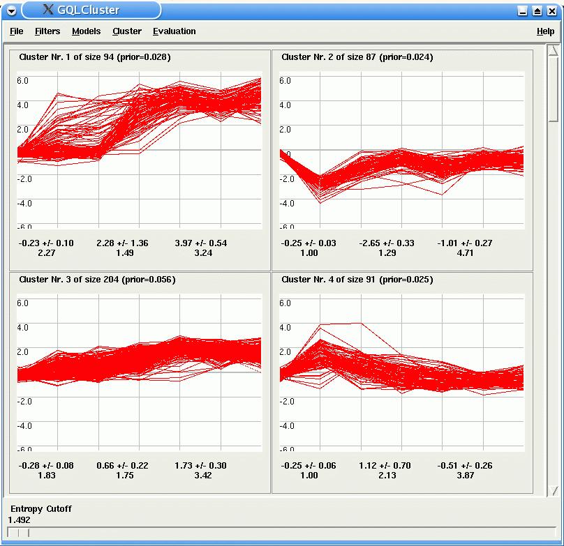
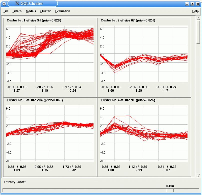
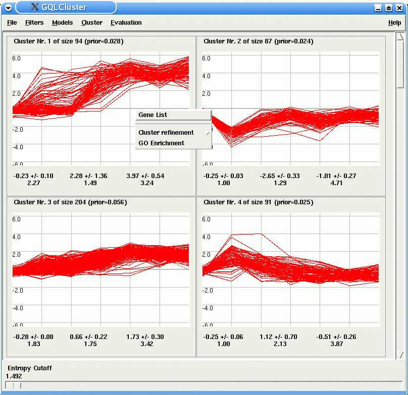
After the estimation, GQLCluster draws, for each HMM, a plot of the time courses assigned to it. Corresponding model parameters are displayed below the time course panels. By using the entropy cutoff bar in the lower part of GQLCLuster, the user can inspect time courses, which were unambigously assigned to only one model.
Data Filtering:
Two common types of time course filtering are implemented and can be accessed through the Filter menu. The n-fold filter accepts only time courses changing more then n folds at least in one time point. The non-constant filter excludes genes where the maximal and minimal values have a difference of at least d.
Initial Model Collection:
The next step is the definition of the initial model collection. The choices to be made for this are: the number of HMMs to be used, and the topology of each of the HMMs, i.e. its number of states (we suggest the use of 30% to 50% of the total number of time points) and its parameters. One way to obtain an initial model collection is to use previously existing models, such as models already defined by the use of GQLQuery. Collection of models can be loaded (or appended to the existing one) through the menu File -> Open Model Set (or Append Model Set).
The user can also choose to generate random models serving as initial collection. For this access the Random Models Dialog with the menu Models -> Random Models.

The number of states field accepts any array definition string in python. For example, '[3]' would define that models should have three states, '[3,5]' that the models should have 3 and 5 states and range(3:5) that models with 3, 4 and 5 should be generated (see python documentation for details on array definitions). The field number of models defines how many copies of the models (given the above states sizes) should be generated. For example, with number of states as '[3,5]' and number of models as 5, five models with three states and five models with five states will be generated. The parameter has two options: the default parameters, which uses default values (defined by default_mean and default_var) to parameterize the HMMs, or the randomize_pars, which obtain random values to parameterize the HMMs.
After generating the models, the users needs to initialize the parameters of the model. GQLCluster offers three distinct forms of estimating the initial model collection. With the Random Assignment Estimation and Random Weights Estimation, each gene is assigned randomly to one model, and a baum welch estimation is carried for each of the models. If partial labels of the data are present, the option Estimate from Partial Assignment can be also be used. In this case, only labeled genes are used in the initialization. In this case, previous to the estimation, the labels should be inputed in GQLCluster, with the menu File -> Open Partial Assignment (see Documentation for file formats)..
GQLCluster also peforms the estimation of the models from the sequence data (menu Models -> Estimate from Sequences). In this case, the user also needs to define the number of states and number of models.
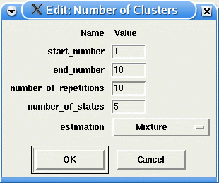
The option Estimate number of Clusters makes uses of BIC to search for the 'optimal' number of clusters in the data set. The user needs to define the initial number of models (start_number) and the final number of models (end_number), the number of estimation repetitions for each model size, the number of states in the models and the type of estimation to be peformed. After all estimations are carried out, GQLCluster displays a graph of BIC X number of clusters, and indicates the 'optimal' number of clusters found (or model size with minimun average BIC value). This procedure is computational intensive and could take some hours for big data sets or high number of clusters.
At any point having generated or provided a set of models, the actual set of their parameters can be inspected and changed, if needed, by use of the menu Models -> Edit. The Edit dialog also allows the user to add or remove HMMs.
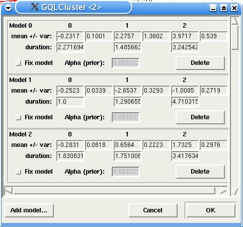
Clustering and Mixture Estimation:
After the successful generation of an initial model collection, the next step is the estimation itself. Three types of estimations are presented: estimate mixture, estimate clustering and estimate mixture with partial labels via the menu Cluster. In all three estimation procedures, the user can set the number of iterations to be performed by the EM algorithm (max_iter), and the stopping criterion (eps), which makes the estimation procedure stop, if changes of the log-likelihood between iterations do not exceed (eps) any more. .

GQLCluster also provides a way of looking at results of old estimations. The user needs only to load the original data set and the estimated collection of models, and select the option Cluster -> View Model Assignment.
Results
For each HMM, GQLCluster display a plot of the time courses assigned to it. In the case of mixture estimation, the slide bar Entropy Cutoff at the bottom of the window, allows the user to select genes which are unambiguously assigned to only one model (the lower the entropy the lower is the ambiguity).
By clicking with the right button over one of the plots, the user can view more detailed information about the clusters, such as the list of time course identifiers with a link to the NCBI Nucleotide database, or look for GO enrichment in the cluster via an external link to GOStat (note that for the successful use of these tools, the identifiers given in the input data set need to be recognized by the linked databases).
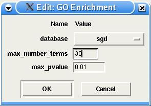
For the GO enrichment, the user must define the annotation database to be searched, the maximum number of GO nodes to be displayed and the maximal p-value. More parameters can later be changed in the GOStat interface.
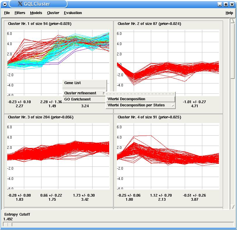
The user can also use the Viterbi Decomposition option to perform a further clustering of genes in a particular HMM. In this case, genes belonging to synchronous sub-groups are plotted in different colors.
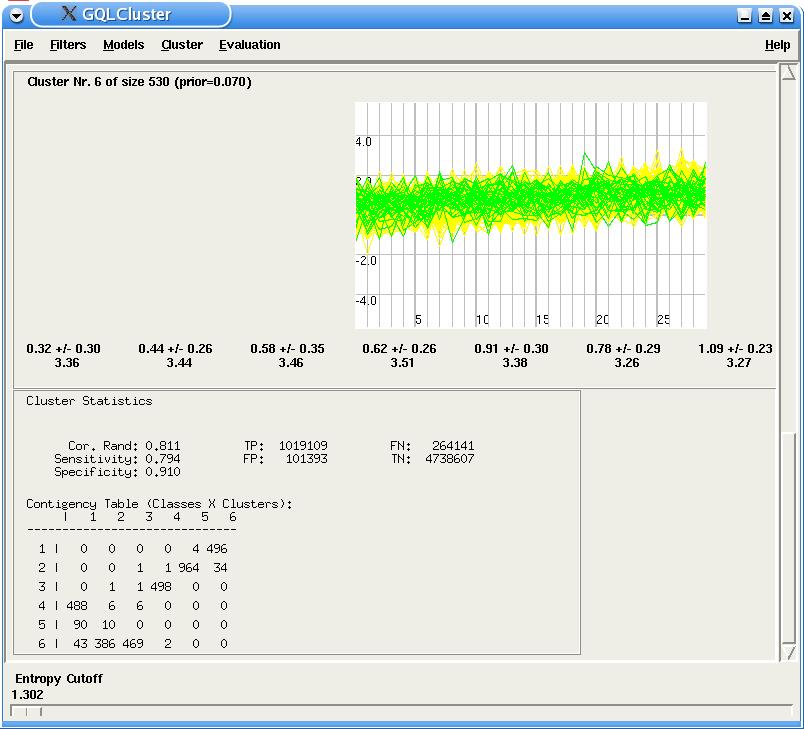
If the user is using a benchmarking data set, i.e. a data set, whose time courses are labeled, GQLCluster is able to supply additional features (the additional information column in the input data set should contain the numerical labeling, such as the one present in the sim1.txt data set). For each class, a distinct color is used to plot the time courses. This way, the user can inspect visually to which model the differently labeled genes were assigned. Moreover a Summary Panel containing a number of corresponding statistics is displayed after below time-courses plots. This panel shows the corrected Rand, sensitivity, specificity and the contingency table (cluster X classes) of the results, and is updated when the entropy cutoff slide is used.
A new feature of GQLCluster allows the user to compare the clustering results with the genes' annotations. Currently, GQLCluster supports only Gene Ontology annotations, but we are working on using protein-protein interaction and regulatory information as well. GQLCluster reads standard GO files, more specifically OBO files for the gene ontology and SGD files for the annotation (definitions of GO and most popular annotations can be found in GO). These files can be loaded in the Menu Evaluation, but notice that the ontology needs to be loaded first. Then make sure that the gene identifiers of the input file match the ones from the GO annotations.
Once the annotation has been loaded and an estimation has been performed, use the menu Evaluation -> Evaluate GO to look for correlations between GO and the results. Since GO is a directed acyclic graph, we need to cut it at some specific level in order to obtain a partition to be compared with the clustering results. The user can define this level in the GO Evaluation dialog (our experience shows that a level of 4 or 5 yields best correlations). In the end, GQLCLuster displays the Summary Panel containing statistics on the comparison of the annotation and the results. This method is still under development and a more precise description of the methods is to be made available soon.
