GQL: Analyzing time-course data

The Graphical Query Language:
A GHMM-based tool for querying and clustering Gene-Expression time-course data

Tutorial GQLQuery

Overview

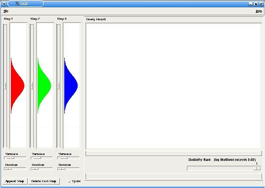
GQLQuery is a graphical interface for querying time course data given a HMM model. The interface is divided in two main parts: the Model panel in the left, where you can see and modify the model's parameters and the Query panel, where information of the queried time courses is displayed.

Getting Started

Run GQLQuery with the following command (or by double-clicking at the executable binary files):

 python GQLQuery.py

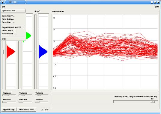
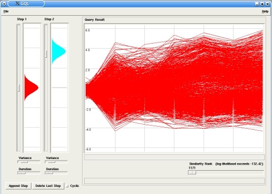
After running GQLQuery, open the file yspo_2fold.txt with the Menu File -> Open Data Set. You will see all available time courses plotted in the Query panel. Next, open the sample model yspo_upregulated.smo in the Menu File -> Open Query. The Model panel is updated to reflect the loaded model parameters (see Documentation for file formats).

Making a Query

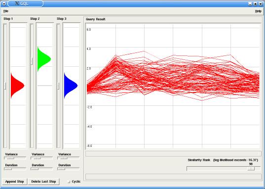
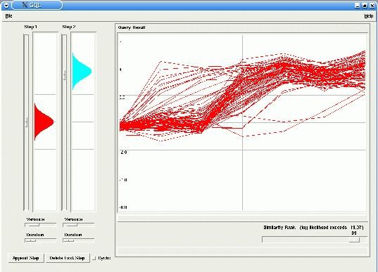
In our example the model has two steps (or states), with probabilities emissions around 0.0 for the first step and around 3.0 for the second step. By changing the similarity rank, using the corresponding slider in the Query panel, only the best fitting time-courses are displayed in the Graph (in this case, up-regulated genes).

The user can also modify the loaded model parameters. Try changing the emission probability of step 2, by changing the slide of step 2 down. If the new emission is negative, only down-regulated genes will be displayed (given that you have set a stringent similarity rank threshold).

Going back to the loaded model, you could also try increasing the duration parameter of step 1, favoring late up-regulated time courses.

New steps can also be included, by clicking in the "Append Step" button in the lower part of the Model panel. For example, add a new step, and make it emit around zero, and (optionally), to sharpen its emissions, lower its variance slide. Now, genes with the behavior non-regulated, up-regulated and non-regulated will be displayed. By adding or deleting new steps, you can try to explore more complex or simple patterns in the data.

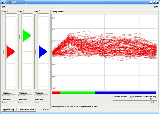
GQLQuery also displays information about the queried genes. By pointing with the mouse cursor over one time course, its identifier or any annotation provided in the data file can be viewed in the lower part of the Query panel. Furthermore, the color bar shown below the plot area, displays in what order the steps of the query are used to generate the respective time-course in the given model (the colors of the bars match with the corresponding step colors).

Saving your Results

After all analysis is done, all results can be saved. Through the Menu File the user can: save the current model, save the current plot in a eps format or create a data file containing only the queried time-courses.